Tutorial
Find your first planet
Recover the giant planet HD 2685 b from public NASA TESS data, measure it, and check it the way professionals do
(Received 8 October 2026)
Using two sectors of public TESS photometry, we recover the hot Jupiter HD 2685 b with a box least squares period search, measure its period, size and orbit, and run the vetting checks that separate a planet candidate from a claim.
Contents
- I.What a transit tells us
- II.Setting up
- III.Finding the data
- IV.Looking at the raw light curve
- V.Cleaning and flattening
- VI.Searching for the period
- VII.Folding the transits
- VIII.Measuring the transit
- IX.From numbers to physics
- X.Vetting the signal
- XI.Checking the neighbours
- XII.Is it already known?
- XIII.From practice to a real search
- XIV.Reporting a candidate
- XV.Working with an AI assistant
- XVI.Sharing on Public Frontier
- References
Run it yourself. Everything below comes from a real run on public NASA data. Download the notebook and open it in Jupyter, or in Google Colab with File → Upload notebook. It runs in a few minutes.
I.What a transit tells us
When a planet passes in front of its star, it blocks a little of the star's light. A telescope that measures the star's brightness every few minutes sees a shallow dip with a flat bottom, repeating once per orbit. That dip is a transit. Three numbers describe it. The period is the time from one transit to the next. The duration is how long each transit lasts. The depth is the fraction of light that disappears, and for a planet much smaller than its star it is close to the ratio of the two disk areas:
where is the radius of the planet and the radius of the star. A planet the size of Jupiter in front of a star the size of the Sun blocks about 1 percent of the light. Earth would block about 0.01 percent.[1][1] Planet Hunters TESS (2026). Project pages and FAQ on Zooniverse, accessed 8 October 2026. zooniverse.org Once we know the mass of the star, the period also gives the size of the orbit through Kepler's third law, and the duration tells us whether the dip makes sense for a body orbiting that star. Winn (2010) derives all of these relations clearly.[2][2] Winn, J. N. (2010). Transits and Occultations. In Exoplanets, ed. S. Seager, University of Arizona Press. arxiv.org
Our target is HD 2685, a star a little hotter and larger than the Sun, about 197 parsecs (640 light-years) away. NASA's Transiting Exoplanet Survey Satellite (TESS) caught the transits of its giant planet in the very first sector of data it took, in 2018. Jones et al. (2019) confirmed the planet with radial-velocity measurements from three spectrographs, which gave it a mass of about 1.2 Jupiter masses, and HD 2685 b became one of the first planets discovered by TESS.[3][3] Jones, M. I., et al. (2019). HD 2685 b: a hot Jupiter orbiting an early F-type star detected by TESS. Astronomy & Astrophysics 625, A16. doi.org It is a hot Jupiter, a gas giant that circles its star in about four days. Small telescopes on the ground follow it too. Observers in the ExoClock project, which anyone with a telescope and a camera can join, have timed six of its transits since 2022.[4][4] ExoClock Project (2026). HD 2685 b planet page and project home page, accessed 8 October 2026. exoclock.space
We chose HD 2685 b because everything about it is clear. The star is bright, the transit is about 1 percent deep, and the four-day orbit gives a dozen transits in two sectors of data. That lets us see each step working before you try it on stars where the answer is unknown.
II.Setting up
You can run everything in a free Google Colab notebook or on your own computer. Download the notebook, open Google Colab, choose File, then Upload notebook, and pick the file. Run the cells from top to bottom. In our runs the whole notebook took between one and four minutes, mostly spent waiting for the archive, and it downloaded about 85 MB of data. A local Jupyter installation works the same way; we used Python 3.12.
The first cell installs Lightkurve, a Python package written for exactly this kind of work with Kepler and TESS data.[5][5] Lightkurve Collaboration (2018). Lightkurve: Kepler and TESS time series analysis in Python. Astrophysics Source Code Library, ascl:1812.013. ascl.net We pin the version so that your numbers match ours:
%pip install -q lightkurve==2.6.0
Lightkurve brings NumPy, Astropy,[6][6] Astropy Collaboration (2022). The Astropy Project: Sustaining and Growing a Community-oriented Open-source Project and the Latest Major Release (v5.0) of the Core Package. The Astrophysical Journal 935, 167. doi.org astroquery,[7][7] Ginsburg, A., et al. (2019). astroquery: An Astronomical Web-querying Package in Python. The Astronomical Journal 157, 98. doi.org SciPy, pandas and Matplotlib with it. The second cell loads them. Lightkurve 2.6 prints a notice about an optional package called oktopus when it starts; it does not affect anything here, so we hide it.
%matplotlib inline
import warnings
warnings.filterwarnings("ignore", message=".*oktopus.*")  # a harmless notice from lightkurve 2.6

import numpy as np
import pandas as pd
import matplotlib.pyplot as plt
import astropy.units as u
import astropy.constants as const
import lightkurve as lk
III.Finding the data
TESS watches a strip of sky 24 degrees wide and 96 degrees long, called a sector, for about 27 days at a time.[8][8] Ricker, G. R., et al. (2015). Transiting Exoplanet Survey Satellite. Journal of Astronomical Telescopes, Instruments, and Systems 1, 014003. doi.org For a selected list of stars it also saves small images every 2 minutes, and the Science Processing Operations Center (SPOC) pipeline at NASA Ames turns them into light curves: tables of brightness against time.[9][9] Jenkins, J. M., et al. (2016). The TESS science processing operations center. Proceedings of the SPIE 9913, 99133E. doi.org Lightkurve asks the Mikulski Archive for Space Telescopes (MAST) for those files:
search = lk.search_lightcurve("HD 2685", mission="TESS", author="SPOC", exptime=120)
print(search)
SearchResult containing 7 data products.

 #     mission     year author exptime target_name distance
                                  s                 arcsec
--- -------------- ---- ------ ------- ----------- --------
  0 TESS Sector 01 2018   SPOC     120   267263253      0.0
  1 TESS Sector 27 2020   SPOC     120   267263253      0.0
  2 TESS Sector 28 2020   SPOC     120   267263253      0.0
  3 TESS Sector 67 2023   SPOC     120   267263253      0.0
  4 TESS Sector 68 2023   SPOC     120   267263253      0.0
  5 TESS Sector 94 2025   SPOC     120   267263253      0.0
  6 TESS Sector 95 2025   SPOC     120   267263253      0.0
TESS has observed HD 2685 at 2-minute cadence in seven sectors between 2018 and 2025. The target_name column is the star's number in the TESS Input Catalog, TIC 267263253. We use sectors 94 and 95, which TESS observed back to back in 2025. Two consecutive sectors give almost two months of nearly continuous data:
recent = lk.search_lightcurve("HD 2685", mission="TESS", author="SPOC", exptime=120, sector=[94, 95])
lcs = recent.download_all()
raw = lcs.stitch()
print(f"{len(raw)} measurements between BTJD {raw.time.value.min():.2f} and {raw.time.value.max():.2f}")
print(f"{len(raw) - len(raw.remove_nans())} of them have no flux value (NaN)")
33752 measurements between BTJD 3856.50 and 3907.54
3098 of them have no flux value (NaN)
stitch() divides each sector by its median brightness and joins them into one light curve. Times are in BTJD, the Barycentric TESS Julian Date. It counts days, corrects them to the centre of mass of the Solar System, and subtracts 2,457,000 to keep the numbers short. The light curve covers 51 days.
IV.Looking at the raw light curve
Figure 1 shows the light curve as SPOC delivers it, using the corrected flux column called PDCSAP. You can draw the same plot with raw.plot(). Twelve dips of about 1 percent stand out at once. So do the gaps: each sector is split into two halves, and the satellite pauses between them to send its data to Earth.
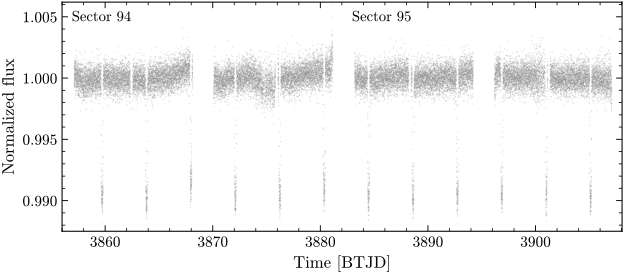
Three kinds of bad data are worth knowing about. First, every measurement carries a quality flag. By default Lightkurve drops measurements that the pipeline flagged for known problems, such as bad calibration, thruster firings that unload the reaction wheels, and stretches the SPOC team excluded by hand. That removed 1,274 of the 18,170 measurements in the sector 94 file and 857 of the 17,713 in sector 95. Second, 3,098 of the remaining measurements have no flux value at all, a NaN (not a number). About 74 percent of them carry a flag for scattered light from the Earth or Moon. Third, single points can jump far from their neighbours, for example when a cosmic ray hits the detector. We deal with the last two in the next step.
V.Cleaning and flattening
Stars drift slowly in brightness, and so does the instrument. A search for transits works best on a light curve where everything except the transits is flat. Lightkurve's flatten() follows the slow trends with a smooth curve (a Savitzky-Golay filter) and divides them out:
lc = raw.remove_nans()
flat = lc.flatten(window_length=901)  # 901 points x 2 minutes = 30 hours
flat = flat.remove_outliers(sigma_lower=np.inf, sigma_upper=4)  # clip upward spikes only
print(f"{len(flat)} measurements left after cleaning")
30654 measurements left after cleaning
The window length decides what counts as a slow trend. Here it is 901 measurements, 30 hours, about seven times longer than a transit. The filter then sees each transit as a brief interruption and passes over it. A window close to the transit length would bend down into every dip and erase part of the signal you are looking for.
We clip outliers on the high side only. A transit is itself a run of low points. The bottom of this transit lies about 13 times the point-to-point scatter below the mean, so a symmetric clip would throw the transits away. For this bright and quiet star the upward clip removed nothing. On fainter or flaring stars it catches cosmic rays and flares.
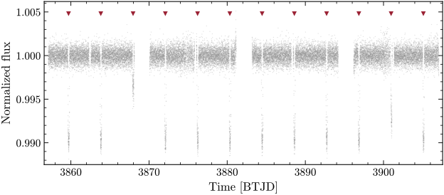
Figure 2 shows a problem we fix later. The two transits next to data gaps, near BTJD 3868 and 3901, came out with depths of 3,143 and 6,767 parts per million (ppm), while the other ten have depths close to 9,500 ppm. Near the end of a stretch of data the filter has little on one side to anchor it, so it bends into the dip.
VI.Searching for the period
Box least squares (BLS) is the standard method for finding periodic transits.[10][10] Kovács, G., Zucker, S., and Mazeh, T. (2002). A box-fitting algorithm in the search for periodic transits. Astronomy & Astrophysics 391, 369. doi.org For every trial period it folds the light curve, so that all the data are placed on one orbit, and slides a box-shaped dip of every trial duration across the fold. The box is flat outside the transit and lower by a constant inside it. BLS records how much better the best box fits the data than a flat line. That score is the BLS power, and the period with the highest power is the best guess.
periods = np.arange(1, 10, 0.001)  # trial periods in days
durations = np.arange(0.04, 0.25, 0.01)  # trial durations in days, about 1 to 6 hours
bls = flat.to_periodogram(method="bls", period=periods, duration=durations)

period = bls.period_at_max_power
t0 = float(bls.transit_time_at_max_power.value)  # mid-transit time in BTJD
duration = bls.duration_at_max_power
depth = bls.depth_at_max_power
print(f"period   = {period.value:.3f} days")
print(f"t0       = {t0:.4f} BTJD")
print(f"duration = {duration.to(u.hour).value:.2f} hours")
print(f"depth    = {depth.value * 100:.3f} %")

power = bls.power.value
sde = (power.max() - power.mean()) / power.std()
print(f"SDE      = {sde:.1f}")
period   = 4.127 days
t0       = 3859.7045 BTJD
duration = 4.13 hours
depth    = 0.844 %
SDE      = 12.8
We tried 9,000 periods from 1 to 10 days and 21 durations from about 1 to 6 hours. The steps must be small enough that the box does not slide off the transits over the 51 days. After 11 orbits, a period wrong by 0.001 days puts the box 16 minutes off, which still sits well inside a transit of 4 hours. The signal detection efficiency (SDE) measures how far the highest peak stands above the rest of the periodogram,
where and are the mean and standard deviation of the power over all trial periods. Here the peak stands 12.8 standard deviations above the average.
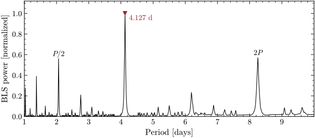
Figure 3 shows the periodogram, drawn with bls.plot() in the notebook. The peak at 4.127 days towers over everything. The peaks at half and twice the period reach 56 and 57 percent of its height. They are echoes: a fold at twice the period still lines up every second transit, and a fold at half the period lines up all of them with an equal number of empty passes in between.
VII.Folding the transits
Now that we know where the transits are, we can fix the damage from Figure 2. We flatten the light curve again and give flatten() a mask that tells it to ignore the transits, so the filter interpolates across them. Then we run BLS once more on a much finer grid around the peak:
mask = lc.create_transit_mask(period=period, transit_time=t0, duration=1.5 * duration)
clean = lc.flatten(window_length=901, mask=mask)
clean = clean.remove_outliers(sigma_lower=np.inf, sigma_upper=4)

zoom = np.arange(period.value - 0.01, period.value + 0.01, 0.00001)
fine = clean.to_periodogram(method="bls", period=zoom, duration=durations)
period = fine.period_at_max_power
t0 = float(fine.transit_time_at_max_power.value)
duration = fine.duration_at_max_power
depth = fine.depth_at_max_power
print(f"period   = {period.value:.5f} days")
print(f"t0       = {t0:.4f} BTJD")
print(f"duration = {duration.to(u.hour).value:.2f} hours")
print(f"depth    = {depth.value * 100:.3f} %")
period   = 4.12662 days
t0       = 3859.7045 BTJD
duration = 4.13 hours
depth    = 0.913 %
With the transits masked, the two damaged transits come back to depths of 9,068 and 9,570 ppm, and the box depth grows from 0.844 to 0.913 percent. Next we fold the light curve at this period, average it in 10-minute bins and overlay the BLS box:
folded = clean.fold(period=period, epoch_time=t0)
binned = folded.bin(time_bin_size=10 * u.min)
model = fine.get_transit_model(period=period, transit_time=t0, duration=duration)
model = model.fold(period=period, epoch_time=t0)

ax = folded.scatter(c="0.7", s=1, label="2-minute data")
binned.scatter(ax=ax, c="k", s=8, label="10-minute bins")
model.plot(ax=ax, c="C3", label="BLS box model")
ax.set_xlim(-0.4, 0.4);
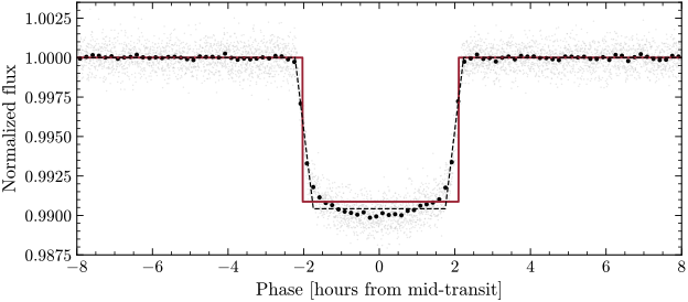
Figure 4 shows a clean transit. It also shows the limits of a box. The real dip has sloped sides, where the planet's disk slides onto and off the star, and a slightly rounded bottom. The box can only be a compromise, so it comes out shorter than the full transit, 4.13 hours, and a little shallower than the middle of the dip.
VIII.Measuring the transit
To measure the transit, we fit a model with sloped sides: a trapezoid. It has five numbers: the mid-transit time , the period , the depth , the total duration (from first to last contact) and the time that the planet takes to cross the edge of the star. SciPy's curve_fit adjusts all five until the model matches the 30,654 measurements as closely as possible, and estimates an uncertainty for each:
from scipy.optimize import curve_fit

def trapezoid(t, t0, period, depth, t14, t12):
    """Flux of a trapezoid transit: total duration t14, ingress and egress t12 each."""
    x = np.abs((t - t0 + period / 2) % period - period / 2)  # days from mid-transit
    flux = np.ones_like(t)
    bottom = x <= t14 / 2 - t12
    edge = (x > t14 / 2 - t12) & (x < t14 / 2)
    flux[bottom] -= depth
    flux[edge] -= depth * (t14 / 2 - x[edge]) / t12
    return flux

guess = [t0, period.value, depth.value, duration.value, duration.value / 10]
low = [t0 - 0.05, period.value - 0.01, 0, 0.02, 0.001]
high = [t0 + 0.05, period.value + 0.01, 0.05, 0.4, 0.1]
t, f, e = clean.time.value, clean.flux.value, clean.flux_err.value
best, cov = curve_fit(trapezoid, t, f, p0=guess, sigma=e, bounds=(low, high))
err = np.sqrt(np.diag(cov))

names = ["t0 [BTJD]", "period [d]", "depth", "t14 [d]", "t12 [d]"]
for name, value, sigma in zip(names, best, err):
    print(f"{name:11s} = {value:.6f} +/- {sigma:.6f}")
T0, P, D, T14, T12 = best
t0 [BTJD]   = 3859.703040 +/- 0.000158
period [d]  = 4.126920 +/- 0.000025
depth       = 0.009580 +/- 0.000021
t14 [d]     = 0.185783 +/- 0.000342
t12 [d]     = 0.020122 +/- 0.000299
The period is now known to about 2 seconds, days, and the transit lasts hours. These uncertainties assume that the noise in each measurement is independent of its neighbours. Real light curves also have slow, correlated wiggles, so treat the error bars as lower limits.
A quick test of the timing: the ExoClock project published an ephemeris for HD 2685 b, a reference transit time and a period, in 2023.[11][11] Kokori, A., et al. (2023). ExoClock Project III: 450 New Exoplanet Ephemerides from Ground and Space Observations. The Astrophysical Journal Supplement Series 265, 4. doi.org Our transit at BJD 2460859.70304 ± 0.00016 comes 517 orbits after their reference transit. Their ephemeris predicts BJD 2460859.70339 ± 0.00053, which is 30 ± 47 seconds later than we measured. The planet is on schedule.
IX.From numbers to physics
To turn the depth into a size we need the size of the star. The TESS Input Catalog (TIC) lists a radius and a mass for every star TESS observes, estimated from Gaia distances, brightness and colour.[12][12] Stassun, K. G., et al. (2019). The Revised TESS Input Catalog and Candidate Target List. The Astronomical Journal 158, 138. doi.org We query it through MAST:
from astroquery.mast import Catalogs

tic = Catalogs.query_object("TIC 267263253", radius=2 * u.arcmin, catalog="TIC")
star = tic[tic["ID"] == "267263253"][0]
R_star = star["rad"] * u.R_sun
M_star = star["mass"] * u.M_sun
print(f"R_star = {star['rad']:.3f} +/- {star['e_rad']:.3f} R_sun")
print(f"M_star = {star['mass']:.2f} +/- {star['e_mass']:.2f} M_sun")
print(f"Teff   = {star['Teff']:.0f} K, distance = {star['d']:.1f} pc")
R_star = 1.587 +/- 0.065 R_sun
M_star = 1.46 +/- 0.25 M_sun
Teff   = 6792 K, distance = 196.9 pc
Three relations do the rest. The planet's radius follows from the depth, . Kepler's third law gives the semi-major axis of the orbit from the period and the star's mass,
where is the gravitational constant. And for a circular orbit seen exactly edge-on, the planet would cross the middle of the star in
If the measured duration came out far from this, the dip could not come from a planet orbiting this star with this period, which makes the duration a first consistency check.
P_d = P * u.day
R_planet = np.sqrt(D) * R_star
a = (const.G * M_star * P_d**2 / (4 * np.pi**2)) ** (1 / 3)
T_central = P_d / np.pi * (R_star / a) * (1 + np.sqrt(D))  # duration if the planet crossed the centre

# simple error propagation
R_planet_err = R_planet * np.hypot(err[2] / (2 * D), star["e_rad"] / star["rad"])
a_err = a * star["e_mass"] / (3 * star["mass"])

print(f"Rp/R*        = {np.sqrt(D):.4f} +/- {err[2] / (2 * np.sqrt(D)):.4f}")
print(f"R_planet     = {R_planet.to(u.R_jup).value:.2f} +/- {R_planet_err.to(u.R_jup).value:.2f} R_jup")
print(f"a            = {a.to(u.au).value:.4f} +/- {a_err.to(u.au).value:.4f} au")
print(f"a / R_star   = {(a / R_star).decompose().value:.2f}")
print(f"central transit would last {T_central.to(u.hour).value:.2f} h, we measured {T14 * 24:.2f} h")
Rp/R*        = 0.0979 +/- 0.0001
R_planet     = 1.51 +/- 0.06 R_jup
a            = 0.0571 +/- 0.0033 au
a / R_star   = 7.74
central transit would last 4.47 h, we measured 4.46 h
HD 2685 b is half again as wide as Jupiter and orbits its star at 0.057 astronomical units, about one seventh of Mercury's distance from the Sun. The measured duration matches a transit across the middle of the star, so the planet passes almost straight across the disk. The table compares our numbers with the published ones. Published values come from Jones et al. (2019), the default parameter set in the NASA Exoplanet Archive,[3, 13][13] Christiansen, J. L., et al. (2025). The NASA Exoplanet Archive and Exoplanet Follow-up Observing Program: Data, Tools, and Usage. The Planetary Science Journal 6, 186. doi.org. Planetary Systems Composite Parameters and TOI tables accessed 8 October 2026, doi.org except the duration, which comes from the TOI catalogue.
| Quantity | This tutorial | Published |
|---|---|---|
| Period [days] | ||
| Radius ratio | ||
| Star radius [] | (TIC) | |
| Star mass [] | (TIC) | |
| Planet radius [] | ||
| Semi-major axis [au] | ||
| Total duration [hours] |
The period agrees within 0.7 standard deviations, and within 0.6 standard deviations of the more precise ExoClock period of 4.126905 ± 0.000001 days.[11] The orbit agrees almost exactly. Our planet radius is 1.51 against 1.44 Jupiter radii, a difference of 0.9 standard deviations, and the reason is worth understanding. Stars look darker towards their edges, an effect called limb darkening. A planet crossing the bright middle of the disk therefore blocks more than its share of the light, so the flat bottom of our trapezoid sits about 7 percent deeper than , and our radius ratio comes out 3 percent too large. The TIC radius of the star is also 2 percent larger than the one Jones et al. derived from spectra. Professional analyses fit a physical transit model that includes limb darkening, for example with the batman package.[14][14] Kreidberg, L. (2015). batman: BAsic Transit Model cAlculatioN in Python. Publications of the Astronomical Society of the Pacific 127, 1161. doi.org For a first measurement from a trapezoid, agreement at this level is what you should expect.
X.Vetting the signal
A periodic dip is a candidate. Many candidates turn out to be something else: two stars eclipsing each other, a faint eclipsing pair blended with a brighter star, or an instrumental effect. Before anyone calls a signal a planet candidate, the TESS pipeline and the TESS team run a standard set of checks on it,[15, 16][15] Twicken, J. D., et al. (2018). Kepler Data Validation I: Architecture, Diagnostic Tests, and Data Products for Vetting Transiting Planet Candidates. Publications of the Astronomical Society of the Pacific 130, 064502. doi.org[16] Guerrero, N. M., et al. (2021). The TESS Objects of Interest Catalog from the TESS Prime Mission. The Astrophysical Journal Supplement Series 254, 39. doi.org and turning a candidate into a confirmed planet takes new observations. Here are the checks you can run yourself.
Odd and even transits. If the dips came from two similar stars eclipsing each other, the true period would be twice what BLS found, and alternate dips could differ in depth because the two stars differ. We measure the depth of the odd-numbered and even-numbered transits separately, using only the flat bottom of each transit and comparing it with the light just before and after:
def drop_ppm(folded_lc, half_width, baseline=(0.6, 1.5)):
    """Mean drop in flux within +/- half_width days of phase zero, in ppm,
    compared with the flux between baseline[0] and baseline[1] transit durations away."""
    x = np.abs(folded_lc.time.value)
    flux = folded_lc.flux.value
    inside = x < half_width
    outside = (x > baseline[0] * T14) & (x < baseline[1] * T14)
    drop = flux[outside].mean() - flux[inside].mean()
    sigma = np.hypot(flux[inside].std() / np.sqrt(inside.sum()),
                     flux[outside].std() / np.sqrt(outside.sum()))
    return drop * 1e6, sigma * 1e6

folded = clean.fold(period=P_d, epoch_time=T0)
bottom = T14 / 2 - T12  # half-width of the flat bottom
odd_depth, odd_err = drop_ppm(folded[folded.odd_mask], bottom)
even_depth, even_err = drop_ppm(folded[folded.even_mask], bottom)
difference = (odd_depth - even_depth) / np.hypot(odd_err, even_err)
print(f"odd transits:  {odd_depth:.0f} +/- {odd_err:.0f} ppm")
print(f"even transits: {even_depth:.0f} +/- {even_err:.0f} ppm")
print(f"difference:    {difference:.1f} sigma")
odd transits:  9514 +/- 43 ppm
even transits: 9613 +/- 38 ppm
difference:    -1.7 sigma
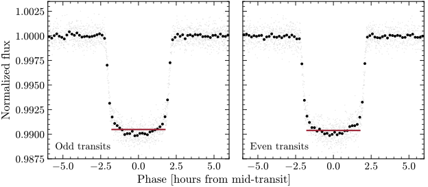
The odd and even depths differ by 99 ppm, 1.7 standard deviations, which is consistent with noise. Figure 5 shows the two sets side by side. This test is also where careless detrending bites. Both transits that the first flattening damaged are even-numbered, so measuring on that light curve would have made the even transits look shallower and faked a difference.
A secondary eclipse at phase 0.5. Halfway between transits the planet passes behind its star. A planet gives off very little light of its own, so almost nothing changes. A companion star of the same size would glow far more, and its eclipse could show up as a second dip at phase 0.5. We fold the light curve with the transit time shifted by half a period and measure the drop there with the same function:
secondary = clean.fold(period=P_d, epoch_time=T0 + P / 2)
eclipse_depth, eclipse_err = drop_ppm(secondary, bottom)
print(f"drop at phase 0.5: {eclipse_depth:.0f} +/- {eclipse_err:.0f} ppm")
drop at phase 0.5: 26 +/- 28 ppm
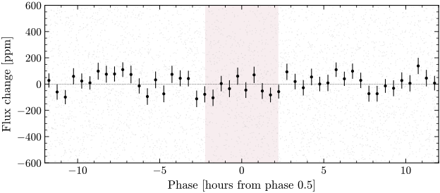
The drop is consistent with zero (Figure 6). At three standard deviations, any eclipse at phase 0.5 is shallower than about 110 ppm, compared with a transit depth of 9,580 ppm. That argues against a glowing companion star. It cannot rule out a brown dwarf, which is about the size of Jupiter and also very dim in TESS's red light. Only a mass settles that question. Jones et al. measured it from the star's wobble in radial velocity: 1.17 Jupiter masses, a planet.[3] Note that an eccentric orbit would move a secondary eclipse away from phase 0.5; HD 2685 b's orbit is close to circular.
The shape of the transit. When a planet much smaller than its star crosses the disk, it slides on and off quickly and spends most of the transit fully in front of the star. The dip has steep sides and a flat floor, a U. When the eclipsing body is large or only grazes the edge of the star, the ingress and egress take up the whole event and the dip looks like a V. The trapezoid fit measures this directly:
print(f"ingress takes {T12 * 24 * 60:.1f} +/- {err[4] * 24 * 60:.1f} minutes")
print(f"that is {T12 / T14:.1%} of the transit; a V-shaped dip would be 50%")
ingress takes 29.0 +/- 0.4 minutes
that is 10.8% of the transit; a V-shaped dip would be 50%
This is a clear U.
XI.Checking the neighbours
Each TESS pixel is 21 arcseconds across,[8] so light from several stars can land in the same pixels. A faint eclipsing binary next to a bright star can mimic a planet transit, because its deep eclipses get diluted by the bright star's light. There is a useful limit to this. A neighbour that is magnitudes fainter than the target contributes a fraction of the target's light, and even if it vanished completely it could not produce a dip deeper than that. So only neighbours with
can be suspects. For a depth of 0.958 percent the limit is 5.0 magnitudes. We list the TIC stars within 2 arcminutes that are bright enough:
faintest = star["Tmag"] - 2.5 * np.log10(D)  # a star fainter than this cannot fake the dip
neighbours = tic[(tic["ID"] != "267263253") & (tic["Tmag"] < faintest)]
print(f"stars within 2 arcmin brighter than Tmag {faintest:.1f}:")
for row in neighbours:
    print(f"  TIC {row['ID']}: Tmag {row['Tmag']:.2f}, {row['dstArcSec']:.0f} arcsec away")
print("share of the aperture light that SPOC assigns to HD 2685:",
      [round(float(one.meta["CROWDSAP"]), 3) for one in lcs])
stars within 2 arcmin brighter than Tmag 14.3:
  TIC 267264183: Tmag 13.58, 67 arcsec away
  TIC 267264184: Tmag 14.01, 69 arcsec away
  TIC 267264180: Tmag 9.91, 80 arcsec away
share of the aperture light that SPOC assigns to HD 2685: [0.978, 0.971]
Three stars qualify, one of them almost as bright as HD 2685 itself. SPOC estimates that 97 to 98 percent of the light inside its photometric aperture comes from HD 2685 and has already corrected the PDCSAP flux for the rest. To see where the light goes missing, we look at the pixels. The target pixel file holds the 11 by 11 pixel images from which the light curve was made. We average the images taken just before and after each transit, subtract the average image taken during the transits, and find the centre of the difference:
tpf = lk.search_targetpixelfile("HD 2685", mission="TESS", author="SPOC", exptime=120, sector=95).download()
x = np.abs((tpf.time.value - T0 + P / 2) % P - P / 2)  # days from mid-transit
during = x < bottom
around = (x > 0.6 * T14) & (x < 1.5 * T14)
image = np.nanmean(tpf.flux[around].value, axis=0)
difference_image = image - np.nanmean(tpf.flux[during].value, axis=0)

def centroid(img):
    """Flux-weighted centre of the 5 x 5 pixels around the brightest pixel."""
    r, c = np.unravel_index(np.nanargmax(img), img.shape)
    rows, cols = np.mgrid[r - 2:r + 3, c - 2:c + 3]
    w = np.clip(img[r - 2:r + 3, c - 2:c + 3], 0, None)
    return (w * cols).sum() / w.sum(), (w * rows).sum() / w.sum()

star_x, star_y = tpf.wcs.world_to_pixel_values(star["ra"], star["dec"])
dip_x, dip_y = centroid(difference_image)
offset = np.hypot(dip_x - star_x, dip_y - star_y)
print(f"the light goes missing {offset:.2f} pixels ({offset * 21:.0f} arcsec) from HD 2685")
the light goes missing 0.12 pixels (3 arcsec) from HD 2685
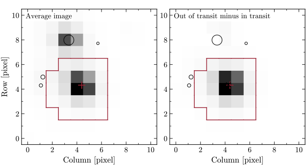
In Figure 7 the bright neighbour shows up clearly in the average image, above the aperture. In the difference image it has vanished, and the missing light sits on HD 2685. The centre of the difference image lies 0.12 pixels, about 3 arcseconds, from the star's catalogue position, while all three suspects lie more than 3 pixels away. The dip comes from HD 2685 or from something within a few arcseconds of it. TESS cannot separate stars closer than that; high-resolution imaging from large ground-based telescopes can.[17][17] TESS Follow-up Observing Program Working Group (2026). TFOP overview and subgroups. tess.mit.edu The SPOC pipeline runs a more careful version of this test, with a model of how TESS images a star, and publishes it in its Data Validation reports.[15] Two free tools help with the same questions for any TESS star: TRICERATOPS computes how likely it is that a signal comes from a nearby star,[18][18] Giacalone, S., et al. (2021). Vetting of 384 TESS Objects of Interest with TRICERATOPS and Statistical Validation of 12 Planets. The Astronomical Journal 161, 24. doi.org and LATTE, written by the Planet Hunters TESS team with citizen scientists in mind, draws these diagnostic plots for you.[19][19] Eisner, N. L., Lintott, C. J., and Aigrain, S. (2020). LATTE: Lightcurve Analysis Tool for Transiting Exoplanets. Journal of Open Source Software 5, 2101. doi.org
XII.Is it already known?
Before you get excited about a signal, check the catalogues. The NASA Exoplanet Archive answers questions written in ADQL, a dialect of SQL, through a public web address.[13] Two queries tell us whether our star is a TESS Object of Interest (TOI) and whether it hosts a confirmed planet:
from urllib.parse import quote

def archive(query):
    """Run an ADQL query on the NASA Exoplanet Archive and return a table."""
    url = "https://exoplanetarchive.ipac.caltech.edu/TAP/sync?format=csv&query="
    return pd.read_csv(url + quote(query))

print(archive("select toi, tfopwg_disp, pl_orbper, pl_trandep, pl_trandurh "
              "from toi where tid = 267263253").to_string(index=False))
print(archive("select pl_name, disc_year, pl_orbper, pl_radj, pl_orbsmax "
              "from pscomppars where tic_id = 'TIC 267263253'").to_string(index=False))
   toi tfopwg_disp  pl_orbper  pl_trandep  pl_trandurh
135.01          CP   4.126905     10831.0        4.405
  pl_name  disc_year  pl_orbper  pl_radj  pl_orbsmax
HD 2685 b       2019    4.12688     1.44      0.0568
HD 2685 b is TOI-135.01, and the TESS Follow-up Observing Program working group (TFOPWG) lists it as CP, a confirmed planet. The TOI catalogue quotes a depth of 10,831 ppm, measured with a different model that includes limb darkening. The ExoFOP page for TIC 267263253 collects everything known about the star in one place. For a new signal you would also search the list of community candidates on ExoFOP and catalogues of variable stars such as the AAVSO's VSX, because many periodic dips belong to known eclipsing binaries.
XIII.From practice to a real search
You have now recovered a planet that you knew was there. A real search looks for signals that nobody has reported, and the first thing to know is how often such signals turn out to be planets. The TOI table records the working group's verdict on every TOI:
counts = archive("select tfopwg_disp, count(*) as n from toi group by tfopwg_disp order by n desc")
print(counts.to_string(index=False))
tfopwg_disp    n
         PC 4824
         FP 1314
         CP  814
         KP  606
        APC  488
         FA  100
        NaN    2
On 8 October 2026 the table held 8,148 TOIs. PC means planet candidate and APC an ambiguous one; together they make up 65 percent, still waiting for a verdict. CP marks planets confirmed after TESS found them and KP planets that were known before; together they make up 17 percent. FP (false positive, a real astrophysical signal that is not a planet) and FA (false alarm, an instrumental or noise signal) make up another 17 percent. Of all the TOIs that have been settled either way, half turned out not to be planets. And TOIs have already survived a strict selection. During the TESS prime mission, vetters inspected 32,814 pipeline detections and promoted 2,241 of them to TOIs, of which 1,676 had not been ruled out as false positives when the catalogue was published.[16] Expect most of your own signals to be something else.
Choosing stars. Start from stars that are not TOIs. The TOI table gives their TIC numbers, and Lightkurve can search around any position. Here we take every star within 2 degrees of HD 2685 that TESS watched at 2-minute cadence in sector 95:
toi_stars = set(archive("select tid from toi")["tid"])
nearby = lk.search_lightcurve("HD 2685", radius=2 * u.deg, mission="TESS", author="SPOC",
                              exptime=120, sector=95)
fresh = nearby[[int(tic_id) not in toi_stars for tic_id in nearby.target_name]]
print(f"{len(nearby)} light curves, {len(fresh)} of them on stars that are not TOIs")
64 light curves, 61 of them on stars that are not TOIs
Searching many light curves. A batch search wraps the steps you already know in a function and runs it on every light curve. We use the first 20 stars to keep the example short:
def quick_search(lc):
    """Flatten a light curve, run BLS and return the best period, depth and SDE."""
    flattened = lc.remove_nans().flatten(window_length=901)
    flattened = flattened.remove_outliers(sigma_lower=np.inf, sigma_upper=4)
    pg = flattened.to_periodogram(method="bls", period=periods, duration=[0.04, 0.08, 0.12, 0.16])
    power = pg.power.value
    result = {"period": pg.period_at_max_power.value,
              "t0": float(pg.transit_time_at_max_power.value),
              "depth_ppm": pg.depth_at_max_power.value * 1e6,
              "sde": (power.max() - power.mean()) / power.std()}
    return result, flattened

rows, flats = [], {}
for i in range(20):
    lc_i = fresh[i].download()
    tic_id = fresh.target_name[i]
    result, flats[tic_id] = quick_search(lc_i)
    rows.append({"tic": tic_id, "Tmag": lc_i.meta["TESSMAG"], **result})
batch = pd.DataFrame(rows).sort_values("sde", ascending=False)
print(batch.drop(columns="t0").round(2).to_string(index=False))
      tic  Tmag  period  depth_ppm   sde
180791583 14.85    1.08   32999.04 10.04
267263040 12.34    9.92    2494.61  6.97
266970549 12.52    8.48    2387.90  6.35
267490189 12.41    1.83    1136.51  6.23
267263797 16.12    4.19   21045.76  6.15
612390067 17.68    8.78  282565.33  5.60
267183188 12.22    5.39    1015.76  5.50
612232178 18.60    9.82  482456.73  5.17
267489655 10.03    8.91     802.81  5.07
267427710 11.94    1.65     520.02  4.96
267046689  7.36    6.12     434.07  4.91
267211524 11.84    1.56     671.27  4.90
266970096 11.85    7.29     630.51  4.79
267091211  4.71    6.75     213.60  4.24
267000601  5.62    3.05     264.59  4.21
181233653  8.18    6.25     528.16  4.12
612256219  2.29    4.47     136.23  4.12
267263203  8.75    6.95     577.76  3.48
267210445  8.46    4.09     586.69  3.39
267211065  2.22    7.17     271.84  3.02
One star stands out, TIC 180791583, with an SDE of 10.0. For comparison, the same quick search on HD 2685 with sector 95 alone gives:
hd_result, _ = quick_search(lcs[1])
print(f"HD 2685, sector {lcs[1].meta['SECTOR']}: period {hd_result['period']:.3f} d, "
      f"depth {hd_result['depth_ppm']:.0f} ppm, SDE {hd_result['sde']:.1f}")
HD 2685, sector 95: period 4.127 d, depth 8960 ppm, SDE 9.9
A real hot Jupiter and a signal that turns out to be no transit at all score almost the same. TIC 180791583 is faint (Tmag 14.85), and the 2-minute scatter in its flattened light curve is 37,636 ppm, larger than the 33,000 ppm "dip" that BLS reports. Folded at its best period, it shows regular waves and no transit shape:
top = batch.iloc[0]
flats[top.tic].fold(period=top.period, epoch_time=top.t0).scatter();
A Lomb-Scargle periodogram, which looks for sine-shaped signals, measures the waves:
ls = flats[top.tic].to_periodogram(method="lombscargle", minimum_period=0.05, maximum_period=5)
print(f"TIC {top.tic} varies by {ls.max_power.value * 100:.1f} % "
      f"every {ls.period_at_max_power.to(u.hour).value:.1f} hours")
TIC 180791583 varies by 1.8 % every 3.7 hours
The star's brightness swings 1.8 percent above and below its average every 3.7 hours, and BLS simply fitted its box into one of the troughs. The lesson is general: a single score cannot tell a planet from noise or from a variable star, so look at the fold of every high scorer and run the vetting checks before you believe anything.
Where new planets hide. SPOC already searches every 2-minute light curve with its own transit search, which flags signals above 7.1 standard deviations.[16] Obvious planets around 2-minute targets are usually TOIs already. Your chances are better with long-period planets that transit only once or twice, which automated searches handle poorly. Of the 90 most promising Planet Hunters TESS candidates in the first two years, 73 showed a single transit.[20][20] Eisner, N. L., et al. (2021). Planet Hunters TESS II: findings from the first two years of TESS. Monthly Notices of the Royal Astronomical Society 501, 4669. doi.org Chances are also better among the far larger number of stars that TESS records only in its full-frame images. MAST hosts light curves for them from the TESS-SPOC and QLP pipelines, and lk.search_lightcurve(..., author="TESS-SPOC") or author="QLP" finds them. Combining many sectors also helps, because shallow signals add up over many transits.
XIV.Reporting a candidate
The rules for reporting a candidate changed in 2026, so check the official pages before you act. ExoFOP, the NASA site where the community shares candidates and follow-up observations, paused new community candidate uploads on 31 March 2026.[21][21] ExoFOP (2026). ExoFOP News, entries of 31 March 2026 and 19 August 2026. NASA Exoplanet Science Institute. exofop.ipac.caltech.edu When it reopened them on 19 August 2026, it added new conditions.[21, 22][22] ExoFOP (2026). Candidate Guidelines. NASA Exoplanet Science Institute. exofop.ipac.caltech.edu A candidate must first be published in a peer-reviewed journal that is available online. A Research Note of the American Astronomical Society also counts, but only if the method used to detect and vet the candidate was already published in a peer-reviewed journal and the note cites it. Uploading requires approval, which you request through ExoFOP's Published Candidate Upload Request form, and the upload must include the paper's URL. A new candidate needs at least two of period, mid-transit time and depth, and the TOI working group only considers TESS candidates that come with all four of period, mid-transit time, depth and duration. Candidates should not get a lowercase planet letter until the refereed literature confirms them.
In practice, a path from your notebook to a reported candidate looks like this:
- Run every check in this tutorial on your signal, in more than one sector if you can, and keep the whole analysis in one notebook that runs from top to bottom.
- Share the notebook and your numbers openly so that others can rerun and question them. Public Frontier exists for this.
- Join Planet Hunters TESS on Zooniverse. The project has been running since December 2018 and is still live. Volunteers mark transits in TESS light curves and discuss them on its Talk boards, and the science team vets the most promising events.[1, 20] Candidates found there have become TOIs before.[16] If you use information from its Talk boards in a publication, the project asks you to cite Eisner et al., contact the team and credit the volunteers involved.[1]
- Write it up. A Research Note of the AAS is at most 1,500 words with one figure or table, is moderated by an editor without peer review, has no author charges at the time of writing, and gets a DOI.[23][23] American Astronomical Society (2026). Research Notes of the AAS: preparation guidelines. journals.aas.org A full peer-reviewed paper usually needs professional collaborators, who can also organise the follow-up observations a confirmation needs.
- Once it is published, request upload access on ExoFOP and submit the candidate with its paper URL, period, mid-transit time, depth, duration and uncertainties, plus a plot of the fitted transit.[22]
If you own a telescope, you can also contribute follow-up observations directly. ExoClock schedules transit observations of known planets for anyone with a telescope and a camera,[4] and the TESS Follow-up Observing Program has a subgroup for ground-based photometry that you can apply to join.[17]
XV.Working with an AI assistant
An AI assistant can make this work much faster, and it can also make you confidently wrong. Use it as a patient tutor and a second pair of eyes. Paste in a cell and its output, and ask it to explain each line until you could rewrite the cell yourself. Ask it which checks you have not run yet, and ask for the code to run them. Then run that code yourself and read the output. Never put a number in your notes, or in a report, that you cannot reproduce by rerunning your notebook, and check every reference it gives you against the archive or the journal page, because assistants invent plausible-looking citations. Two prompts that work well:
Here is a notebook cell and its output. Explain what each line does in plain words, and tell me which results depend on choices I made, such as the window length or the period grid. Suggest one way to test whether those choices change my answer.
My BLS search found a 1.08-day signal with SDE 10 on TIC 180791583, a star of TESS magnitude 14.9. List the checks I should run before calling it a candidate, in order, and write Lightkurve code for the first one. Do not quote any numbers about this star that I have not given you.
XVI.Sharing on Public Frontier
When your notebook runs cleanly from top to bottom, put it in a public GitHub repository with a short README that names the star, the TESS sectors and the package versions you used. Anyone can then open it in Google Colab straight from GitHub, at an address of the form colab.research.google.com/github/<user>/<repository>/blob/main/<notebook>.ipynb.
Then share it as a discovery note. Sign in with an email address or a Bluesky handle, write a title and a short abstract, upload your folded light curve as a figure, and fill in the period, mid-transit time, depth and duration you measured. For this tutorial, set the status to Known object recovered. A recovery shows that your pipeline works, and others can compare their numbers with yours. Add the links to your repository and notebook, and say how you used AI. The note is stored in your own ATProto repository, and anyone can rerun your analysis and comment on it.
References
- [1]Planet Hunters TESS (2026). Project pages and FAQ on Zooniverse, accessed 8 October 2026. https://www.zooniverse.org/projects/nora-dot-eisner/planet-hunters-tess
- [2]Winn, J. N. (2010). Transits and Occultations. In Exoplanets, ed. S. Seager, University of Arizona Press. https://arxiv.org/abs/1001.2010
- [3]Jones, M. I., et al. (2019). HD 2685 b: a hot Jupiter orbiting an early F-type star detected by TESS. Astronomy & Astrophysics 625, A16. https://doi.org/10.1051/0004-6361/201834640
- [4]ExoClock Project (2026). HD 2685 b planet page and project home page, accessed 8 October 2026. https://www.exoclock.space/database/planets/HD2685b/
- [5]Lightkurve Collaboration (2018). Lightkurve: Kepler and TESS time series analysis in Python. Astrophysics Source Code Library, ascl:1812.013. https://ascl.net/1812.013
- [6]Astropy Collaboration (2022). The Astropy Project: Sustaining and Growing a Community-oriented Open-source Project and the Latest Major Release (v5.0) of the Core Package. The Astrophysical Journal 935, 167. https://doi.org/10.3847/1538-4357/ac7c74
- [7]Ginsburg, A., et al. (2019). astroquery: An Astronomical Web-querying Package in Python. The Astronomical Journal 157, 98. https://doi.org/10.3847/1538-3881/aafc33
- [8]Ricker, G. R., et al. (2015). Transiting Exoplanet Survey Satellite. Journal of Astronomical Telescopes, Instruments, and Systems 1, 014003. https://doi.org/10.1117/1.JATIS.1.1.014003
- [9]Jenkins, J. M., et al. (2016). The TESS science processing operations center. Proceedings of the SPIE 9913, 99133E. https://doi.org/10.1117/12.2233418
- [10]Kovács, G., Zucker, S., and Mazeh, T. (2002). A box-fitting algorithm in the search for periodic transits. Astronomy & Astrophysics 391, 369. https://doi.org/10.1051/0004-6361:20020802
- [11]Kokori, A., et al. (2023). ExoClock Project III: 450 New Exoplanet Ephemerides from Ground and Space Observations. The Astrophysical Journal Supplement Series 265, 4. https://doi.org/10.3847/1538-4365/ac9da4
- [12]Stassun, K. G., et al. (2019). The Revised TESS Input Catalog and Candidate Target List. The Astronomical Journal 158, 138. https://doi.org/10.3847/1538-3881/ab3467
- [13]Christiansen, J. L., et al. (2025). The NASA Exoplanet Archive and Exoplanet Follow-up Observing Program: Data, Tools, and Usage. The Planetary Science Journal 6, 186. https://doi.org/10.3847/PSJ/ade3c2. Planetary Systems Composite Parameters and TOI tables accessed 8 October 2026, https://doi.org/10.26133/NEA13
- [14]Kreidberg, L. (2015). batman: BAsic Transit Model cAlculatioN in Python. Publications of the Astronomical Society of the Pacific 127, 1161. https://doi.org/10.1086/683602
- [15]Twicken, J. D., et al. (2018). Kepler Data Validation I: Architecture, Diagnostic Tests, and Data Products for Vetting Transiting Planet Candidates. Publications of the Astronomical Society of the Pacific 130, 064502. https://doi.org/10.1088/1538-3873/aab694
- [16]Guerrero, N. M., et al. (2021). The TESS Objects of Interest Catalog from the TESS Prime Mission. The Astrophysical Journal Supplement Series 254, 39. https://doi.org/10.3847/1538-4365/abefe1
- [17]TESS Follow-up Observing Program Working Group (2026). TFOP overview and subgroups. https://tess.mit.edu/followup/
- [18]Giacalone, S., et al. (2021). Vetting of 384 TESS Objects of Interest with TRICERATOPS and Statistical Validation of 12 Planets. The Astronomical Journal 161, 24. https://doi.org/10.3847/1538-3881/abc6af
- [19]Eisner, N. L., Lintott, C. J., and Aigrain, S. (2020). LATTE: Lightcurve Analysis Tool for Transiting Exoplanets. Journal of Open Source Software 5, 2101. https://doi.org/10.21105/joss.02101
- [20]Eisner, N. L., et al. (2021). Planet Hunters TESS II: findings from the first two years of TESS. Monthly Notices of the Royal Astronomical Society 501, 4669. https://doi.org/10.1093/mnras/staa3739
- [21]ExoFOP (2026). ExoFOP News, entries of 31 March 2026 and 19 August 2026. NASA Exoplanet Science Institute. https://exofop.ipac.caltech.edu/tess/news.php
- [22]ExoFOP (2026). Candidate Guidelines. NASA Exoplanet Science Institute. https://exofop.ipac.caltech.edu/tess/candidate_help.php
- [23]American Astronomical Society (2026). Research Notes of the AAS: preparation guidelines. https://journals.aas.org/research-note-preparation-guidelines/
Finished? Share what you found, even if it is a known planet: share a discovery. A recovery shows your pipeline works, and that is where every search starts.